How Does Batch Normalization Work? Part 2¶

batch-norm

In Part 1, we saw that batch normalization (BN) can help train neural networks by reducing internal covariate shift (ICS) and smoothing gradient updates. We measured ICS as distributional shift in layer activations, in line with Ioffe and Szegedy (2015). For a fully-connected network with 4 layers, we observed that the activation distributions with BN were comparatively stable compared to those for the network without BN. We also touched upon the idea that BN has a smoothing effect on the loss surface, making it more convex.

In their 2018 paper, Santurkar et al. argued that the reduction in internal covariate shift due to BN is marginal at best, and might even increase it. Additionally:

BN improves training performance even when random noise is added to the layer activations, forcing ICS. Therefore, ICS is independent of the effectiveness of BN.
Using a new, gradient-based definition of ICS, they showed that BN has no substantial effect on it, and might even increase it.
The effectiveness of BN, including other desirable effects like preventing vanishing/exploding gradients as well as robustness to initialization and hyperparameter choices are merely downstream effects of an underlying set of causes:
- Lower Lipschitzness of the (i.e. smoother) loss surface.
- Lower Lipschitzness of the gradients i.e. better gradient predictiveness and consequently, higher “effective” \(\beta\)-smoothness of the gradients.
- More favourable initialization.

In this experiment, we will attempt to reproduce some of these findings.

Let’s Start by Downloading and Preprocessing the Dataset¶

The CIFAR-10 dataset includes 60,000 color images of size 32×32 pixels, divided into 50,000 training images and 10,000 testing images. The dataset is organized into ten distinct classes: airplane, automobile, bird, cat, deer, dog, frog, horse, ship, and truck.

To save some space, I have written a CIFAR-10 dataloader which downloads and performs standard preprocessing (normalization and augmentation). For this experiment, we will not augment the dataset.

from deepkit.datasets import load_CIFAR10

train_loader, test_loader = load_CIFAR10(augment=False)

Let’s Set Up the Baseline and Candidate Models¶

We’ll be using a VGG-Net style network with 10 3x3 convolutional and 3 FC layers including the final classifier. The activations are ReLU. The candidate model has a BatchNorm layer after each convolutional layer. The weights for both networks are initialized using the Glorot/Xavier method, which is standard for convolutional networks. To simplify our analysis, we will not use any regularization like dropout or weight decay.

import jax
import jax.numpy as jnp
import flax.nnx as nnx

kernel_init = nnx.initializers.glorot_normal()


class VGGBlock(nnx.Module):
    def __init__(self, in_features: int, out_features: int, rngs: nnx.Rngs):
        self.conv = nnx.Conv(in_features=in_features,
                             out_features=out_features,
                             kernel_size=(3, 3),
                             kernel_init=kernel_init,
                             padding='SAME',
                             rngs=rngs)
        self.bn = nnx.BatchNorm(num_features=out_features, momentum=0.90, rngs=rngs)

    def __call__(self, x):
        x = self.conv(x)
        x = self.bn(x)
        conv_activation = x
        x = nnx.relu(x)
        return x, conv_activation

class VGGNet(nnx.Module):
    def __init__(self, rngs: nnx.Rngs):
        self.convs = [
            VGGBlock(in_features=3, out_features=64,  rngs=rngs),
            VGGBlock(in_features=64, out_features=64,  rngs=rngs),

            VGGBlock(in_features=64, out_features=128, rngs=rngs),
            VGGBlock(in_features=128, out_features=128, rngs=rngs),

            VGGBlock(in_features=128, out_features=256, rngs=rngs),
            VGGBlock(in_features=256, out_features=256, rngs=rngs),

            VGGBlock(in_features=256, out_features=512, rngs=rngs),
            VGGBlock(in_features=512, out_features=512, rngs=rngs),

            VGGBlock(in_features=512, out_features=512, rngs=rngs),
            VGGBlock(in_features=512, out_features=512, rngs=rngs),
        ]

        self.fc1 = nnx.Linear(in_features=512, out_features=96, kernel_init=kernel_init, rngs=rngs)
        self.fc2 = nnx.Linear(in_features=96, out_features=96, kernel_init=kernel_init, rngs=rngs)
        self.out = nnx.Linear(in_features=96, out_features=10,  kernel_init=kernel_init, rngs=rngs)

    def __call__(self, x):
        activations = {}
        max_pool_after = [1, 3, 5, 7, 9]
        for conv_idx in range(len(self.convs)):
            layer = self.convs[conv_idx]
            x, act = layer(x)
            activations[f"conv_{conv_idx}"] = act
            if conv_idx in max_pool_after:
                x = nnx.max_pool(x, window_shape=(2, 2), strides=(2, 2))

        x = x.squeeze()

        x = self.fc1(x)
        activations["fc1"] = x
        x = nnx.relu(x)

        x = self.fc2(x)
        activations["fc2"] = x
        x = nnx.relu(x)

        x = self.out(x)
        activations["out"] = x
        return x, activations

Let’s initialize the baseline (non-BN) and candidate (BN) models. Both networks are initialized with the same random key for consistency and reproducibility. Both networks have roughly 9.5 million paramters.

rng_key = jax.random.key(1337)
rngs = nnx.Rngs(rng_key)
candidate = VGGNet(rngs=rngs)
candidate_graphdef, candidate_state = nnx.split(candidate)
param_counts = sum(jax.tree_util.tree_leaves(jax.tree_util.tree_map(lambda x: x.size,
                                                                    candidate_state)))
print(f"Initialized model with {param_counts:,} parameters.")
nnx.display(candidate_state)

The Flax-NNX library makes it quite easy to modify models. To remove the BN layers, we can simply set them to the identity function.

rng_key = jax.random.key(1337)
rngs = nnx.Rngs(rng_key)
baseline = VGGNet(rngs=rngs)

# Remove the batchnorm layers
for vgg in baseline.convs:
  vgg.bn = lambda x: x

baseline_graphdef, baseline_state = nnx.split(baseline)
param_counts = sum(jax.tree_util.tree_leaves(jax.tree_util.tree_map(lambda x: x.size,
                                                                    baseline_state)))
print(f"Initialized model with {param_counts:,} parameters.")
nnx.display(baseline_state)

We’ll be using standard stochastic gradient descent with momentum to simplify the analysis and isolate the effects of batch normalization. The learning rate is tuned to be as high as can be sustained by the non-BN network without diverging.

import optax

lr = 0.035
momentum = 0.9

baseline_optimizer = nnx.Optimizer(baseline, optax.sgd(learning_rate=lr, momentum=momentum,
                                                       nesterov=False))
candidate_optimizer = nnx.Optimizer(candidate, optax.sgd(learning_rate=lr, momentum=momentum,
                                                         nesterov=False))

The loss is measured using cross-entropy, which is standard for multi-label classification. Accuracy is measured on both the train and test datasets and tracked through the training run.

from functools import partial

def loss_fn(model, batch, targets):
    logits, activations = model(batch)
    loss = optax.softmax_cross_entropy_with_integer_labels(logits, targets).mean()
    return loss, activations

@nnx.jit
def step_fn(model: nnx.Module, optimizer: nnx.Optimizer, batch: jax.Array, labels: jax.Array):
    (loss, activations), grads = nnx.value_and_grad(loss_fn, has_aux=True)(model, batch, labels)
    optimizer.update(grads)
    return loss, activations, grads


@nnx.jit
def accuracy(model: nnx.Module, batch: jax.Array, labels: jax.Array):
    logits, _ = model(batch)
    preds = jnp.argmax(logits, axis=-1)
    sum = jnp.sum(preds == labels)
    acc = sum/logits.shape[0]
    return acc


def test_accuracy(model: nnx.Module, testloader):
    acc, n = 0, 0
    for batch, labels in testloader:
        batch = jnp.array(batch)
        labels = jnp.array(labels)
        acc += accuracy(model, batch, labels)
        n += 1
    return acc/n

The number of epochs is set to 39, which is roughly 15000 training steps.

from deepkit.loggers import DiskLogger


num_epochs = 39
num_steps = num_epochs*len(train_loader)

Let’s Set Up the Training Loop¶

The training loop is quite involved because we need to calculate and track all the measurements. At each step, the internal covariate shift, loss landscape smoothness and gradient predictiveness calculations are performed for both models. Both the baseline and candidate models are trained in the same loop.

Both the gradient predictiveness and loss Lipschitzness maximum steps are capped at roughly 0.7 times the gradient.

I have moved the measurements to a separate library Deepkit to save some space here.

from deepkit.internal_covariate_shift import (
    santurkar_ics_step,
    loss_landscape_step,
    grad_landscape_step
)

from matplotlib import pyplot as plt
plt.style.use('seaborn-v0_8-darkgrid')
from IPython.display import clear_output

%matplotlib inline

max_step=20
landscape_step_size=2
grad_step_size=2

try:
  for epoch in range(num_epochs):
      for batch, labels in train_loader:
          batch = jnp.array(batch)
          labels = jnp.array(labels)

          baseline_optimizer_copy = baseline_optimizer.__deepcopy__()
          baseline.train()
          baseline_loss, baseline_activations, baseline_grads = (
              step_fn(baseline, baseline_optimizer, batch, labels)
          )
          baseline_train_losses.append(baseline_loss)

          # Calculate ICS
          baseline_optimizer_copy.model.eval()
          baseline_ics_measures = santurkar_ics_step(baseline_optimizer_copy,
                                           baseline_grads,
                                           batch,
                                           labels)
          baseline_ics_results.append(baseline_ics_measures)

          # Calculate loss landscape
          baseline_copy = baseline.__deepcopy__()
          baseline_copy.eval()
          baseline_loss_range = (
              loss_landscape_step(baseline_copy,
                                  batch,
                                  labels,
                                  baseline_grads,
                                  max_step=max_step,
                                  step_size=landscape_step_size,
                                  lr=lr
             )
          )
          baseline_loss_landscape_ranges.append(baseline_loss_range)

          # Calculate gradient predictiveness
          baseline_grad_range = (
              grad_landscape_step(baseline_copy,
                                  batch,
                                  labels,
                                  baseline_grads,
                                  max_step=max_step,
                                  step_size=grad_step_size,
                                  lr=lr
             )
          )
          baseline_grad_landscape_ranges.append(baseline_grad_range)


          candidate_optimizer_copy = candidate_optimizer.__deepcopy__()
          candidate.train()
          candidate_loss, candidate_activations, candidate_grads = (
              step_fn(candidate, candidate_optimizer, batch, labels)
          )
          candidate_train_losses.append(candidate_loss)

          # Calculate ICS
          candidate_optimizer_copy.model.eval()
          candidate_ics_measures = santurkar_ics_step(candidate_optimizer_copy,
                                           candidate_grads,
                                           batch,
                                           labels)
          candidate_ics_results.append(candidate_ics_measures)

          # Calculate loss landscape
          candidate_copy = candidate.__deepcopy__()
          candidate_copy.eval()
          candidate_loss_range = (
            loss_landscape_step(candidate_copy,
                                batch,
                                labels,
                                candidate_grads,
                                max_step=max_step,
                                step_size=landscape_step_size,
                                lr=lr
             )
          )
          candidate_loss_landscape_ranges.append(candidate_loss_range)

          # Calculate gradient predictiveness
          candidate_grad_range = (
            grad_landscape_step(candidate_copy,
                                batch,
                                labels,
                                candidate_grads,
                                max_step=max_step,
                                step_size=grad_step_size,
                                lr=lr
             )
          )
          candidate_grad_landscape_ranges.append(candidate_grad_range)


          baseline.eval()
          baseline_acc = accuracy(baseline, batch, labels)
          baseline_train_accs.append(baseline_acc)

          candidate.eval()
          candidate_acc = accuracy(candidate, batch, labels)
          candidate_train_accs.append(candidate_acc)

          if i % 200 == 0:
            baseline_test_acc = test_accuracy(baseline, test_loader)
            candidate_test_acc = test_accuracy(candidate, test_loader)
            baseline_test_accs.append(baseline_test_acc)
            candidate_test_accs.append(candidate_test_acc)
            baseline_activations_logger.log(i, baseline_activations)
            candidate_activations_logger.log(i, candidate_activations)
          if i % 20 == 0:
            clear_output(wait=True)
            print(f"iter: {i} | baseline loss: {baseline_loss:0.4f} | "
                  f"candidate loss: {candidate_loss:0.4f} | "
                  f"baseline train acc: {baseline_acc:0.2f} | "
                  f"candidate train acc: {candidate_acc:0.2f} | "
                  f"baseline test acc: {baseline_test_acc: 0.2f} | "
                  f"candidate test acc: {candidate_test_acc: 0.2f}")
            fig, axes = plt.subplots(1, 3, figsize=(15, 4))
            axes[0].plot(baseline_train_losses, alpha=0.9,
                         label="Without BatchNorm")
            axes[0].plot(candidate_train_losses, alpha=0.5,
                         label="With BatchNorm")
            axes[0].set_title("Loss")
            axes[0].set_xlabel("Iteration")
            axes[1].plot(baseline_train_accs, alpha=0.9,
                         label="Without BatchNorm")
            axes[1].plot(candidate_train_accs, alpha=0.5,
                         label="With BatchNorm")
            axes[1].set_title("Train Accuracy")
            axes[1].set_xlabel("Iteration")
            x = list(range(len(baseline_test_accs)))
            x = [ i*200 for i in x ]
            axes[2].plot(x, baseline_test_accs, label="Without Batchnorm")
            axes[2].plot(x, candidate_test_accs, label="With Batchnorm")
            axes[2].set_title("Test Accuracy")
            axes[2].set_xlabel("Iteration")
            plt.legend()
            plt.show()

          i += 1
except KeyboardInterrupt:
    print("Received KeyboardInterrupt. Exiting...")

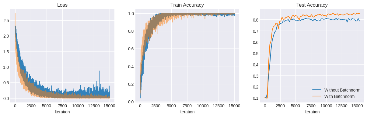
iter: 15040 | baseline loss: 0.0136 | candidate loss: 0.0010 | baseline train acc: 0.99 | candidate train acc: 1.00 | baseline test acc:  0.79 | candidate test acc:  0.85

_images/c319d480dc223fbb69a83d35f7a0d6bdf9846079182d330fa0de2f160adef442.png

Received KeyboardInterrupt. Exiting...

Performance¶

The BN network clearly performs better than the non-BN one - it converges faster and achieves a higher accuracy on the test set - 85% vs 80% for the non-BN network.

Next, let’s analyze the measurements that we gathered during the training process.

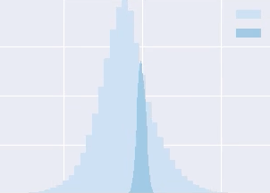
Ioffe et. al ICS i.e. Distributional Shift of the Activations¶

First, let’s plot the activation distributions. From the plots below, it is clear that the BN activations are initally more widely distributed due to BN scaling. However, this changes quickly as training progresses - they remain more stable than the non-BN ones. This matches the results that we obtained back in Part 1. It also seems to contradict the findings of Santurkar et al. (2018), which will require further investigation.

Santurkar et al. ICS i.e. Gradient Shift¶

Rather than the activations themselves, this definition measures the change in gradient norms for each layer before and after the previous layers are updated:

Mathematically, internal covariate shift (ICS) of activation \(i\) at time \(t\) is defined as \(||G_{t,i} − G^′_{t,i}||^2\), where \( \begin{align} G_{t,i} &= ∇_{W^{(t)}_i} \mathcal{L}(W_{1}^{(t)},..., W^{(t)}_k ; x(t), y(t)) \\ G^′_{t,i} &= ∇_{W^{(t)}_i} \mathcal{L}(W^{(t+1)}_1 ,..., W^{(t+1)}_{i−1}, W^{(t)}_i, W^{(t)}_{i+1},..., W^{(t)}_k; x(t), y(t)). \end{align} \)

This is more of an operational definition that measures the impact on the gradient of a particular layer due to covariate shift. It is useful because the gradient is ultimately what impacts learning - a sensitive loss landscape may cause a significant change in the gradient of a layer even without significant changes in its inputs. Conversely, a less sensitive loss landscape may cause little change in the gradient inspite of significant changes to the inputs.

_images/184b11a922a01ce8c0290606d8d8cf85eb96504e6a024fddc947b36b99e029a5.png

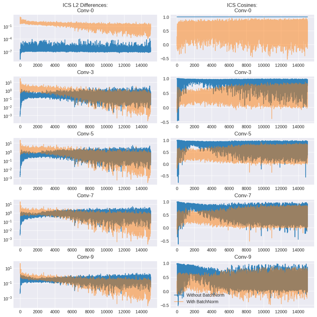
Ideally, the L2 differences (\(||G_{t,i} − G^′_{t,i}||^2\)) should be \(0\) while the cosines \(\frac{\langle G_{t,i},G^′_{t,i}\rangle}{||G_{t,i}||||G^′_{t,i}||}\) should be 1, indicating zero covariate shift.

The left column of the plots above indicates the gradient L2 differences for each layer. The results look inconclusive - the BN model has higher values earlier in the training run, while the non-BN plot has higher values later. The right column measures the cosine values for each convolutional layer. The cosine values for the BN model tend to be lower (i.e. worse) consistently compared to the non-BN one.

One way to interpret these results would be that despite the lower distributional ICS due to BN, the impact on gradient ICS isn’t obvious. This might be because the underlying cause for the effectiveness of BN is not ICS, but the smoothing effect on the loss landscape itself.

Loss Landscape Smoothness i.e. Lipschitzness¶

Lipschnitzness can be considered as a tight upper bound on the steepness of a function. It is defined as:

\(|| f(x) - f(y) || \leq L|| x - y ||\) for all \(x,y \in \mathbb{R}^n\)

where \(L\) is the Lipschitz constant.

If \(f(x)\) is the loss function, smaller \(L\) indicates a ‘flatter’ loss surface. This is hard to measure because it involves an intractable computation over all pairs \((x, y)\). However, we can approximate it by taking a few steps in the gradient direction at every point in the optimization trajectory and measuring \(|| f(x^`) - f(x) ||\) at each step.

In simple terms, a bumpy loss surface should show larger variation in the loss values along the optimization trajectory, while a smoother one should show smaller variation.

_images/be7c2f522aaf3418feaa6d2bd97fece48fafa0752a8d6c36ba382be55f23a846.png

From the above plot, it is clear that the non-BN model shows significantly higher Lipschitzness throughout the training run.

Gradient Predictiveness¶

Lipschitzness can be defined for the gradient as well and can be approximated by how much the L2 norm of the gradient changes in the gradient direction at a point \(x\). This is also called gradient predictiveness. This comes from the idea that a more predictive gradient should remain stable and not change significantly in the gradient direction.

“Effective” \(\beta\)-Smoothness¶

This follows the notion of gradient predictiveness above. Similar to Lipschitzness, \(\beta\)-smoothness provides a tight upper bound on the rate of change of the gradient. A smaller rate of change indicates a smoother loss surface. Formally,

\(|| \nabla f(x) - \nabla f(y) || \leq \beta || x - y || \quad \text{for all } x, y \in \mathbb{R}^n \)

Once again, this is an intractable calculation, so we can approximate it at each point in the optimization trajectory by taking a few steps in the gradient direction and recording the maximum change in the gradient norm.

_images/8e283763281ae9fc486c4b40005a5014490f38eba02961d4da10e2ba380632ec.png

Again, it is clear that gradient predictiveness for the BN network is consistently better (lower is better) throughout the training run. Note that this is a log plot, so each y-tick in an order of magnitude. It is especially clear towards the end of the training run when the BN model’s L2 gradient difference goes to 0 while the non-BN network’s remains high.

More Favorable Initialization¶

BN leads to more favourable initialization for the weights. Mathematically,

\( || W_0 - \hat{W}^∗ ||^2 ≤ ||W_0 − W^∗||^2 − \frac{1}{||W^∗||^2} ( ||W^∗||^2 −〈W^∗, W_0〉)^2 \)

where \(W_0\) is the initial weights and \(\hat{W}^*\) and \(W^*\) are the nearest local minima for the BN and non-BN networks respectively. The proof for this result is available in Santurkar et. al (2018).

We can test this empirically by measuring the L2 differences between the initial weights and the optima for both networks.

_images/5769a97c8c7406ec7db8a6339e4e07fc4529cf78cf1680db3cec60d0a1358dc8.png

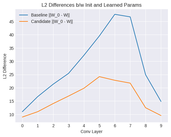
As seen in the plot above, the value is consistently smaller for the BN network for all the convolutional layers. indicating that an optimum is located much closer to the initialization in terms of Euclidean distance for the BN model.

Conclusion and Future Work¶

According to the distributional shift definition of ICS, (Ioffe et al. (2015)), we can observe a significant reduction in ICS due to BN, which appears to contradict the results obtained by Santurkar et al. However, using the Santurkar et al. definition of ICS as gradient shift, it is not as clear. In some cases, it appears to worsen it. From the loss landscape measurements, it is clear that BN has a smoothing effect on the loss surface, improves gradient predictiveness and leads to more favorable initialization. These might be the more fundamental reasons behind its efficacy.

In the next experiment, we will examine the effect of adding random noise to the layer activations as well as try to reconcile the results for the distributional ICS measurement (the effect of BN on distributional ICS may be secondary and largely independent of the performance of BN). We will also delve into the math behind the smoothing theory.

References¶

Santurkar, S., Tsipras, D., Ilyas, A., & Madry, A. (2018). How does batch normalization help optimization? Advances in Neural Information Processing Systems, 31. https://arxiv.org/abs/1805.11604
Ioffe, S., & Szegedy, C. (2015). Batch normalization: Accelerating deep network training by reducing internal covariate shift. In Proceedings of the 32nd International Conference on Machine Learning (ICML) (pp. 448–456). https://arxiv.org/abs/1502.03167
Simonyan, K., & Zisserman, A. (2014). Very deep convolutional networks for large-scale image recognition [Preprint]. arXiv. https://arxiv.org/abs/1409.1556